
Let’s generate random non-overlapping polygons on a plane! Sounded fairly simple to me at the beginning, but soon I discovered those nasty polygons are not as innocent as I thought.
I originally had an idea to explore another optimization problem. I don’t want to write much about it as I’ll probably cover it in a future post but as a first step to it, I had to be able to cover a square area with random non-overlapping polygons. I was mainly interested in equally covering the whole plane (more or less) with many shapes that don’t overlap. Other than that, I didn’t care much and expected it to be fairly simple, although not trivial. Luckily enough, Prof. Dan Halperin works in the office right next to me. He showed me a paper he wrote on Minikowski Sum, and some of the random polygons they generated there proved me that I don’t really want random polygons. Random polygons also include holes, crosses and polygons with 200 vertices that just look like an overkill for me.
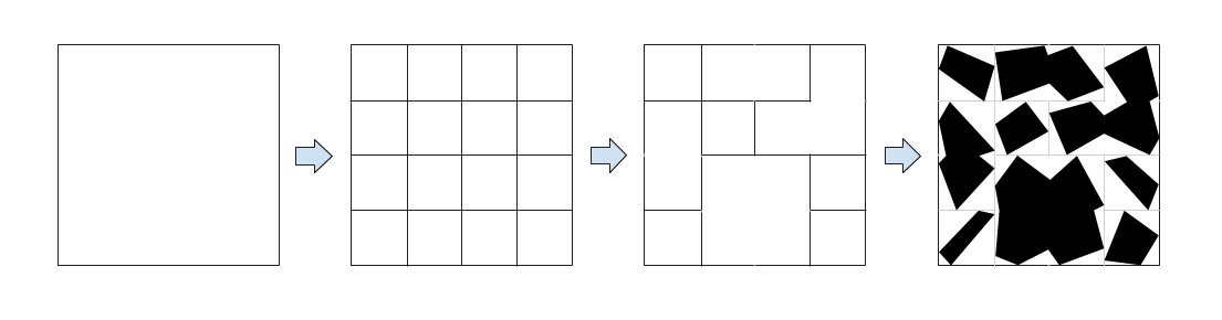
So I went with a second approach - why not considering the square area as a large grid, remove some of the boundaries between adjacent cells to create randomly shaped blocks, and then, draw exactly one polygon inside every block. Given a block, drawing the polygon inside shouldn’t be that difficult and although this approach doesn’t cover all possible polygons, it’s much simpler, straight-forward and ensures me full coverage, non-overlapping and polygons that look more like what ordinary people expect them to.
In high level, it will look something like this:
There are two main factors to play with:
- N - the size of the grid (NxN)
- p - the probability of a separator between two cells to exist
Step 1: Generating a Random Grid
Generating a grid inside the square is pretty simple. Making it a Random Grid shouldn’t be a difficult task for anyone with more than 5 minutes experience in any programming language. Just iterate over all separators and remove them with a probability 1-p.
I didn’t feel comfortable enough with p as it’s not very intuitive. I felt like the user should at least be able to get the feeling of what an average block size would be while he plays with different values for p so I started looking for an expression for the number of blocks (or the average block size) in a grid of size NxN when p is the probability for a separator.
I finally used \( \left[ \frac{ (1-p)^N(Np-p+2) + p - 2 }{ p } \right]^2 \) as the expression for the average block size by N and p. It’s not accurate, but gives an estimation that is fairly OK for our purpose considering that we’re mainly interested in large N and p around 0.7-0.8 (large grids and a lot of the separators in place). You can play with different N and p in the example below.
Developing this expression was really nice (at least I think so..) but involved some math that some might find as scary (it’s really basic, but sometimes gets long and ugly). If you want to see how I got this (and you should!), scroll down to the Random Grid Expression Drill Down section. For simplicity I’ll continue assuming this estimation works.
Step 2: From Blocks to Polygons
Given a set of blocks, we want to draw a polygon in every block so every polygon preserves the shape of the block (that was randomly created) and doesn’t get out of the block so we get the non-overlapping property for free. I could draw a squarish polygon inside every block, but that would be boring. Instead, I had the following pseudo-code in mind:
for block in blocks:
    polygon = []

    for separator in block.separators:
        point = separator.randomizePoint()
        point.addPadding()

        if (nonConvexTurn()):
            polygon.push(cornerPoint)

        polygon.push(point)

    polygon.draw()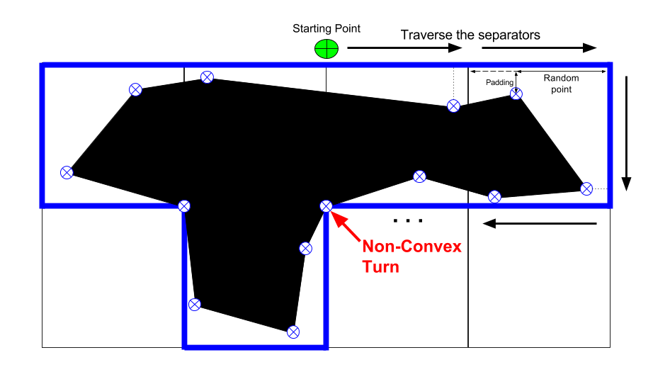
Notice that we must take care of the ‘non-convex’ turns. Otherwise, a line drawn straight between those two points will cross another cell and may overlap with the polygon that is there.
I implemented something like this pseudo-code in Javascript. I officially hate this programming language now! I really don’t see why they need to get to the 6th version of the language (ECMA6, not supported yet in most browsers) to add equality operator override and Array utilities, but whatever.. It’s done now and you can see it below.
Example
Below is an example for generating random polygons using the algorithm described. You can play with N to change the grid size, p to change the separator’s probability and get an estimation of the block size. Good luck!
Random Grid Expression Drill Down
Our goal in this (long) section will be to explain the expression for the average block size in a random grid of size NxN with a separator probability of p as shown before.
First, I’ll note that while the original problem came from the world of grids, tiles and separators, one can easily transform the grid to a graph (where every cell is a vertex), the separators to edges (where every two cells that are not separated are connected with an edge) and therefore ask: how many connected components are there in a Random Graph with a probability p for an edge.
The only difference, and apparently that’s a big one, is that a grid is not a regular graph and not every vertex can be connected to all the others. Only those who are adjacent on the grid can have an edge between them. While I’ve found some (pretty complicated) theorems on number of connected components for a general random graph, I couldn’t find anything that I’ll be able to convert to the grid use-case (aka a Lattice Graph) and so I decided to try and get an estimation on my own.
Reducing to a Random Row
A grid, as being a two-dimensional object, is not a very simple one for combinatorics calculations. I tried to tackle it from different angles and decided the best would be to reduce the problem to something more convenient.
A simpler version of a grid would be a single row. If we can find an expression that ties together block sizes, N and p for a single row, it might be easier to get the more generic grid case from there. Basically, we are looking on the following problem:
What’s the expected number of blocks of size K in a row of size N with p as the probability for a separator?
\(E_N(k) = ?\)
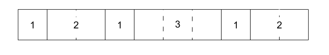
In the example above, we have 3 blocks of size 1, 2 blocks of size 2 and 1 of size 3. We want to express the expected (on average) number of blocks of any size by N and p.
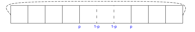
Reducing Again to a Cyclic Row
A ‘regular’ row is very annoying as well because the first and last cells are different from the others (have only one adjacent cell). If we want to consider the probability for a block to start on the 1st cell, we can assume there is no neighbor on the left, but in other cells we’ll have to restrict the left separator to be in place. I tried two ways to overcome this. One was writing an expression for an infinite row and then ‘look’ only on part of it (otherwise all expected numbers are ∞). The other, which is what I moved on with, was to look on a cyclic row (a row where the rightmost separator actually separates the last and the first cell).
This assumptions is clearly not in the original problem, but we can assume it is minor, and for large N it won’t make a difference (2 different cells out of a 100 don’t affect much the number of blocks of size 5..). At the end, when we’ll have an expression based on a cyclic row, it’ll be worth checking how well it estimates a regular row.
Let’s define \( X_i^k \) to be a random variable that gets the following values:
\[
X_i^k=
\begin{cases}
1 & \text{if a block of size } k \text{ starts at cell } i \\\
0 & \text{otherwise}
\end{cases}
\]
We denoted before \( E_N(k) \) as the expected number of blocks of size k in a cyclic row of size N. Because the row is cyclic and blocks can start at the end and span to the beginning, the random variable for the number of blocks of size k in a row should simply be \( \sum\limits_{i=1}^N{X_i^k} \).
Here’s the tricky part - Although \(X_i \)s are statistically dependent on each other (i.e. if a block of size 3 starts at the 1st cell, another one can’t start on the 2nd cell as well), \( E_N(k) \) is the expected value of the sum of them, and from the Linearity of Expectation property we get:
\[
\begin{align}
E_N(k) & = E \left( \sum\limits_{i=1}^N { X_i^k } \right) \\
& = E(X_1^k) + E(X_2^k) + \cdots + E(X_N^k) &&\text{from linearity of expectation} \\
& = P(X_1^k) + P(X_2^k) + \cdots + P(X_N^k) &&\text{X gets 0 or 1 with probability P}\\
& = NP(X) &&\text{from symmetry - all P’s are the same}
\end{align} \\
\text{(Where } P(X) \text{ is the probability for a block of size } k \text{)}
\]
Let’s look on P(X). If p is the probability for a separator, we need 2 separators on both sides of the block, and then another (k-1) in the middle. Therefore, \( P(X) = p^2(1-p)^{k-1} \) and that makes:
\[ E_N(k) = Np^2(1-p)^{k-1} \]
The exception to that is when \( k = N \). In that case, there are no two separators at all so the whole expression is wrong. In order to get a block that fills the whole row, you can either have only one separator somewhere in the row (P(X) will be \( p(1-p)^{N-1} \) and we can have it in N places), or none at all (and then P(X) will be \( (1-p)^N \) and can only appear in one place as no matter where you start this combination of separators, you’ll get the same block). So if we try to express \( E_N(k) \) more accurately, it’s going to be like:
\[
E_N(k) = \begin{cases}
Np^2(1-p)^{k-1} & k<N\\
Np(1-p)^{N-1} + (1-p)^N & k=N
\end{cases}
\]
Given that expression, the expected number of blocks in a row would be a summation of the expected number of blocks for any possible length (i.e. 1..N). We’ll denote that as \(B_N\):
\[
\textbf{NUMBER OF BLOCKS} = B_N = Np + (1-p)^N
\]
The total number of blocks in a row is the sum of all possible blocks: \[ \begin{align} B_N & = \sum\limits_{i=1}^N E_N(i) \\ & = \sum\limits_{i=1}^{N-1}{ E_N(i) } + E_N(N) \\ & = \sum\limits_{i=1}^{N-1}{ Np^2(1-p)^{i-1}} + Np(1-p)^{N-1} + (1-p)^N \\ & {\scriptsize \text{Notice that the summation is the sum of a geometric series with } a_1=Np^2 \text{ and } q=1-p } \\ & = \frac{Np^2(1-(1-p)^{N-1})}{p} + Np(1-p)^{N-1} + (1-p)^N \\ & = Np - Np(1-p)^{N-1} + Np(1-p)^{N-1}+ (1-p)^N \\ & = Np + (1-p)^N \end{align} \]
Verify the \(E_N(k) \) Expression for a Cyclic Row
As we defined, \( E_N(k) \) is an expression for how the expected number of blocks of size k in a row of size N depends on p. Obviously, the total size of all blocks in a row should be N so the following equation should hold:
\[
\sum\limits_{i=1}^N{ i E_N(i) } = N
\]
First, let’s look on the general summation of \( iX^i \):
\[
\begin{align}
\sum\limits_{i=1}^N { iX^i } & = X + 2X^2 + 3X^3 + 4X^4 + \cdots \\
& = X(1 + 2X + 3X^2 + 4X^3 + \cdots) \\
& = X[X + X^2 + X^3 + X^4 + \cdots]’ \\
& = X \left[ \frac{ a_1(1-q^n) }{ 1-q } \right]’ = X \left[ \frac{ X(1-X^N )}{ 1-X } \right]’ \\
& = X \left[ \frac{ NX^{N+1}-(N+1)X^N+1 }{ (X-1)^2 } \right]
\end{align} \\[10pt]
\]
Derivatives thanks to WolframAlpha
And, for the specific summation we’re after:
\[
\require{cancel}
\begin{align}
\sum\limits_{i=1}^N{ i E_N(i) } & = \sum\limits_{i=1}^{N-1}{ i E_N(i) } + NE_N(N) \\
& = \sum\limits_{i=1}^{N-1}{ iNp^2(1-p)^{i-1}} + N^2p(1-p)^{N-1} + N(1-p)^N \\
& = \frac{ Np^2 }{ 1-p }\sum\limits_{i=1}^{N-1}{ i(1-p)^i } + N^2p(1-p)^{N-1} + N(1-p)^N \\
& { \scriptsize \text{Using the general expression from before. Notice that } N=N-1 \text{ and } X=(1-p)} \\
& = \frac{ N\cancel{p^2} }{ \cancel{1-p}} \cdot \frac{ \cancel{(1-p)} \left[ (N-1)(1-p)^N - N(1-p)^{N-1} + 1 \right] }{ \cancel{(1-p-1)^2} } + N^2p(1-p)^{N-1} + N(1-p)^N \\
& = N(N-1)(1-p)^N - N^2(1-p)^{N-1} + N + N^2p(1-p)^{N-1} + N(1-p)^N \\
& = N(1-p)^{N-1} \left[ (N-1)(1-p) - N + Np + (1-p) \right] + N \\
& = N(1-p)^{N-1} \left[ (N-1)(1-p) + (-N+1)(1-p) \right] + N \\
& = N
\end{align}
\]
Another thing we can do is to simulate many random cyclic rows, count the number of blocks and compare to the estimator we got here. Ohh, how lucky I am to know python (code is here).
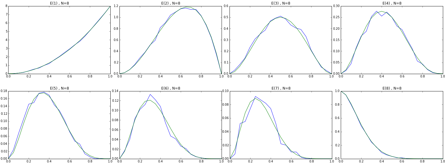
The following graphs shows \( E_8(k) \) (N=8, k=1..8) by p. The blue line is the average number of blocks in 1000 iterations and the green line is the estimated number based on the expression above. I think we’ve nailed the cyclic row!
Verify the Cyclic Assumption
Just as a reminder, we started with the ‘cyclic assumption’ because we assumed that for large values of N, the average number of blocks of a ‘regular’ row and a cyclic one will converge. It’s also important to mention that for the original purpose of this problem, we want to divide the square into a fairly dense grid (N~100 at least).
Let’s run some tests to verify that the assumption holds for rows and grids. If you want, you can continue running the python notebook to get the following graphs. Notice that the grid simulation might take some time…
Verify the Cyclic Assumption for a Row
The python code iterates over values of N (from 5 to 250) and for every one, iterates over all p’s and averages the total number of blocks (\( B_N \)) for 50 iterations. It does it twice. Once with the RegularRow object and the other with CyclicRow. The average absolute difference between them is divided by N to normalize the results. We basically get the error in % by N.
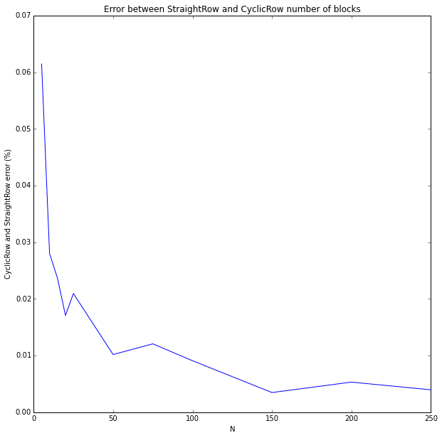
It’s less than 1% for large N’s which is completely acceptable for my problem.
Verify the Cyclic Assumption for a Grid
More or less the same, only now the two classes being compared are StraightGrid and CyclicGrid. The error is normalized by N squared (number of cells). Notice that N’s are much smaller this time, just because grids are heavier to compute (for many N’s, many p’s and many iterations…). You can run it for larger N’s. I felt it’s enough as it is.
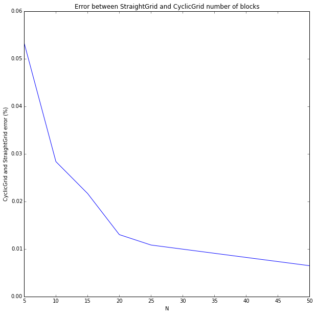
We’ve shown that both for a row, and for a grid, the cyclic assumption doesn’t affect the estimator much when we are dealing with large N’s.
Write the Expression for a Cyclic Grid
Just to recap, we already have the following expressions:
- The expected number blocks in a row for every size of a block - \( E_N(k) \), where k is the block size
- The expected total number of blocks in a row - \( B_N \)
All expressions are by N and p.
In the previous section we’ve looked at the bias we have in the model (we’ve built it for a cyclic row although our rows are actually regular ones) and we are fairly satisfied with it.
We want to do the same for a 2D grid. First, like before, we’ll reduce the problem to a cyclic grid. It had worked once, and we saw it’s safe to use even for grids, so why not try this again?
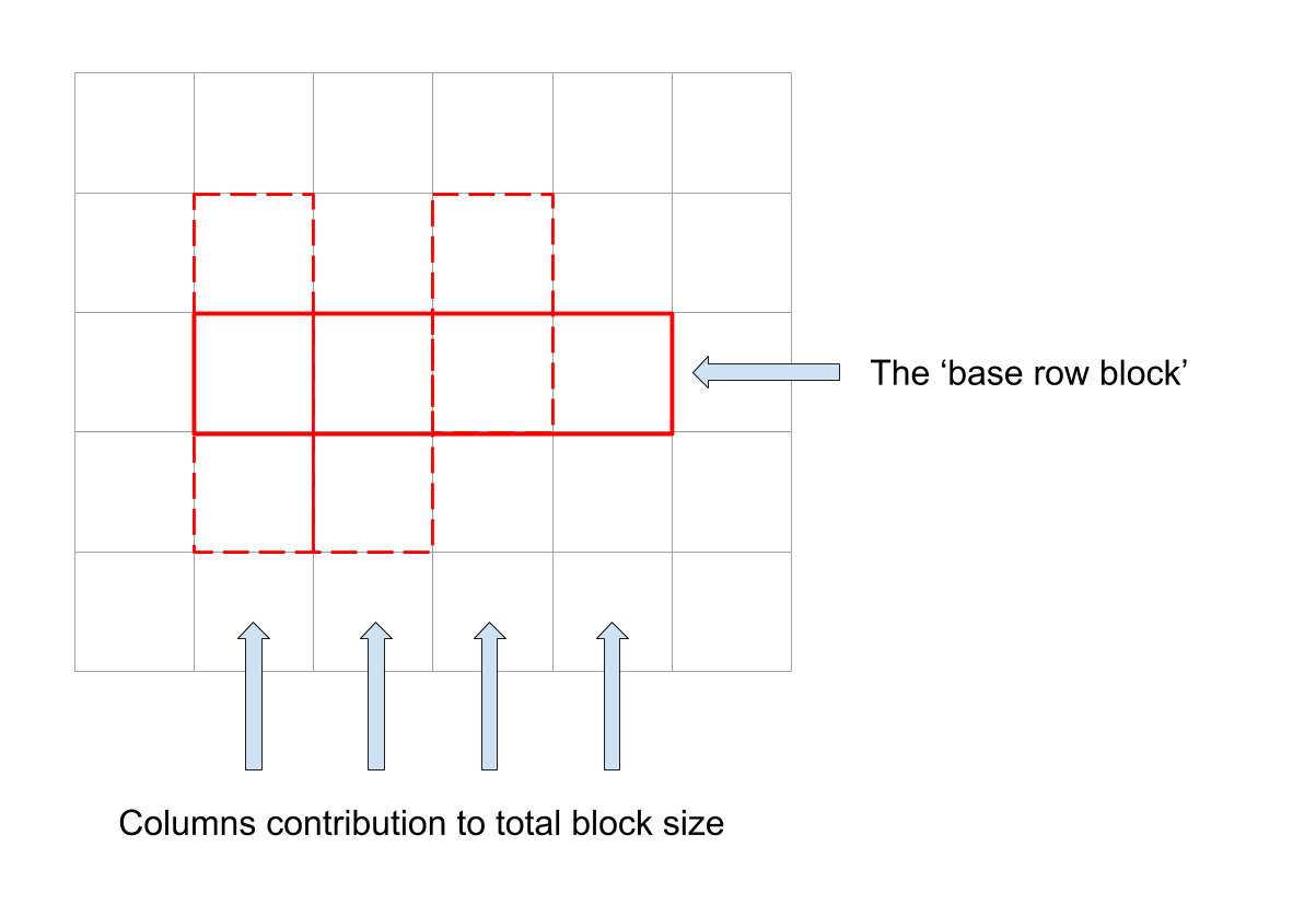
For simplicity, we’ll assume that all blocks have some sort of a ‘base row’ of an arbitrary length and every cell in that row is a part of a column of an arbitrary length. Our block size is then the summation of all columns sizes.
Obviously this is very simplistic and doesn’t cover all cases. I prefer using this assumption because although here I do expect to see a difference between the actual performance and the estimator for a block’s size, I hope that for large p’s it will be acceptable. The rational is that if p is close to 1.0, most separators are in place and we are less likely to get to ‘crazy’ blocks that doesn’t fit this model.
Don’t get me wrong. This assumption is way weaker than the cyclic one and will almost certainly add bias to our estimator. We use it because without it it would have been a combinatorical nightmare to deal with all possible block’s sizes (and because it’s late and I want to go to sleep..).
Every cell has a probability of \( \frac{ iE_N(i) }{N} \) to be in a row block of size i. That’s because the nominator is the number of cells that belong to i size blocks and the denominator is obviously the number of cells in a row. Therefore, if we choose a random cell in a row, it’s expected block size will be \( \sum\limits_{i=1}^N { \frac{ i^2 E_N(i) }{N} } \) .
The total block size is the weighted average of sizes of the ‘base row block’ multiplied by the expected column size. Because rows and columns are equal, we can use the same expression as before for the expected column size.
\[
\underbrace{
\sum\limits_{i=1}^N{
{\huge[}
\frac{i E_N(i)}{N}
\cdot
\underbrace{
i
\cdot
\underbrace{
\sum\limits_{j=1}^N{
\frac{ j^2 E_N(j) }{N}
}
}_{\text{ Average contribution of a column }}
}_{\text{Multiplied by the number of columns in a block (the row block size)}}
{\huge]}
}
}_{\text{Weighted averaged by the probability for such a block}}
\]
And that clearly equals:
\[
\left[ \frac{ (1-p)^N(Np-p+2) + p - 2 }{ p } \right]^2
\]
First, recall our proof from before that: \[ \sum\limits_{i=1}^N { iX^i } = X + 2X^2 + 3X^3 + 4X^4 + \cdots = \cdots = \frac{ NX^{N+2}-(N+1)X^{N+1}+X }{ (X-1)^2 } \] Then, in a similar way, let’s look at: \[ \begin{align} \sum\limits_{i=1}^N{ i^2 X^i } & = X + 4X^2 + 9X^3 + 16X^4 + … \\ & = X \left[ 1 + 4X + 9X^2 + 16X^3 + \cdots \right] \\ & = X \left[ X + 2X^2 + 3X^3 + 4X^4 + \cdots \right]’ \\ & = X \left[ \frac{ NX^{N+2}-(N+1)X^{N+1}+X }{ (X-1)^2 } \right]’ \\ & = X \left[ \frac{ (-2N^2-2N+1)X^{N+1} + N^2X^{N+2} + (N+1)^2X^N-X-1} { (X-1)^3 } \right] \\ & = \frac{ (-2N^2-2N+1)X^{N+2} + N^2X^{N+3} + (N+1)^2X^{N+1}-X^2-X} { (X-1)^3 } \end{align} \] Derivative thanks to WolframAlpha The next step would be: \[ \begin{align} \sum\limits_{i=1}^N{ i^2 E_N(i) } & = \sum\limits_{i=1}^{N-1}{ i^2E_N(i) } + N^2 E_N(N) \\ & = \sum\limits_{i=1}^{N-1}{ i^2 Np^2(1-p)^{i-1} } + N^2 \left[ Np(1-p)^{N-1} + (1-p)^N \right] \\ & = \frac{ Np^2 }{1-p } \cdot \sum\limits_{i=1}^{N-1}{ \left[ i^2 (1-p)^i \right] } + N^3p(1-p)^{N-1} + N^2(1-p)^N \\ & = \frac{ Np^2 }{1-p } \cdot \frac{ \left( -2(N-1)^2-2(N-1) + 1 \right)(1-p)^{N+1} + (N-1)^2(1-p)^{N+2} + N^2(1-p)^N - (1-p)^2 - (1-p) }{ (1-p-1)^3 } + N^3p(1-p)^{N-1} + N^2(1-p)^N \\ & = \cdots \\ & = -\frac{N}{p} \left[ (1-p)^N(Np-p+2) + p - 2 \right] \end{align} \] This huge expression was compactified with WolframAlpha. May god bless them for saving me a couple of days.. And finally: \[ \text{Average Block Size in a Grid = } \\ \begin{align} \sum\limits_{i=1}^N { \left[ \frac{ i^2 E_N(i) }{ N } \cdot \sum\limits_{j=1}^{N} { \frac{ j^2 E_N(j) }{N} } \right] } & = \frac{1}{N^2} \cdot \sum\limits_{i=1}^N{ i^2 E_N(i) } \sum\limits_{j=1}^N{ j^2 E_N(j) } \\ & = \frac{1}{\cancel{N^2}} \left[ -\frac{\cancel{N}}{p} \left( (1-p)^N(Np-p+2) + p - 2 \right) \right] ^ 2 \\ & = \left[ \frac{ (1-p)^N(Np-p+2) + p - 2 }{ p } \right]^2 \end{align} \] Told ya’
I’m using this exact expression to evaluate and represent the block size when the user plays with values of p in the example at the beginning of the post.
A Nice Observation on the Expression
If we look on this expression in Desmos and play with the slider for N we can see that although the expression depends on both N and p, when we increase N, the value for relatively large p’s (\( 0.5 \le p \le 1.0 \)) doesn’t change at all.
This is a nice observation and we could have actually expected to get something like it. If p is large, the chances for a lot of adjacent separators to be missing and create a large block are negligible, so blocks tend to be small, and by that - not bounded by the grid size. The thing that limits the block size (for large p’s) is the probability for a separator and not the hard limit of the grid itself. This of course wont hold for a grid of 3x3 but we don’t look on those cases anyway..
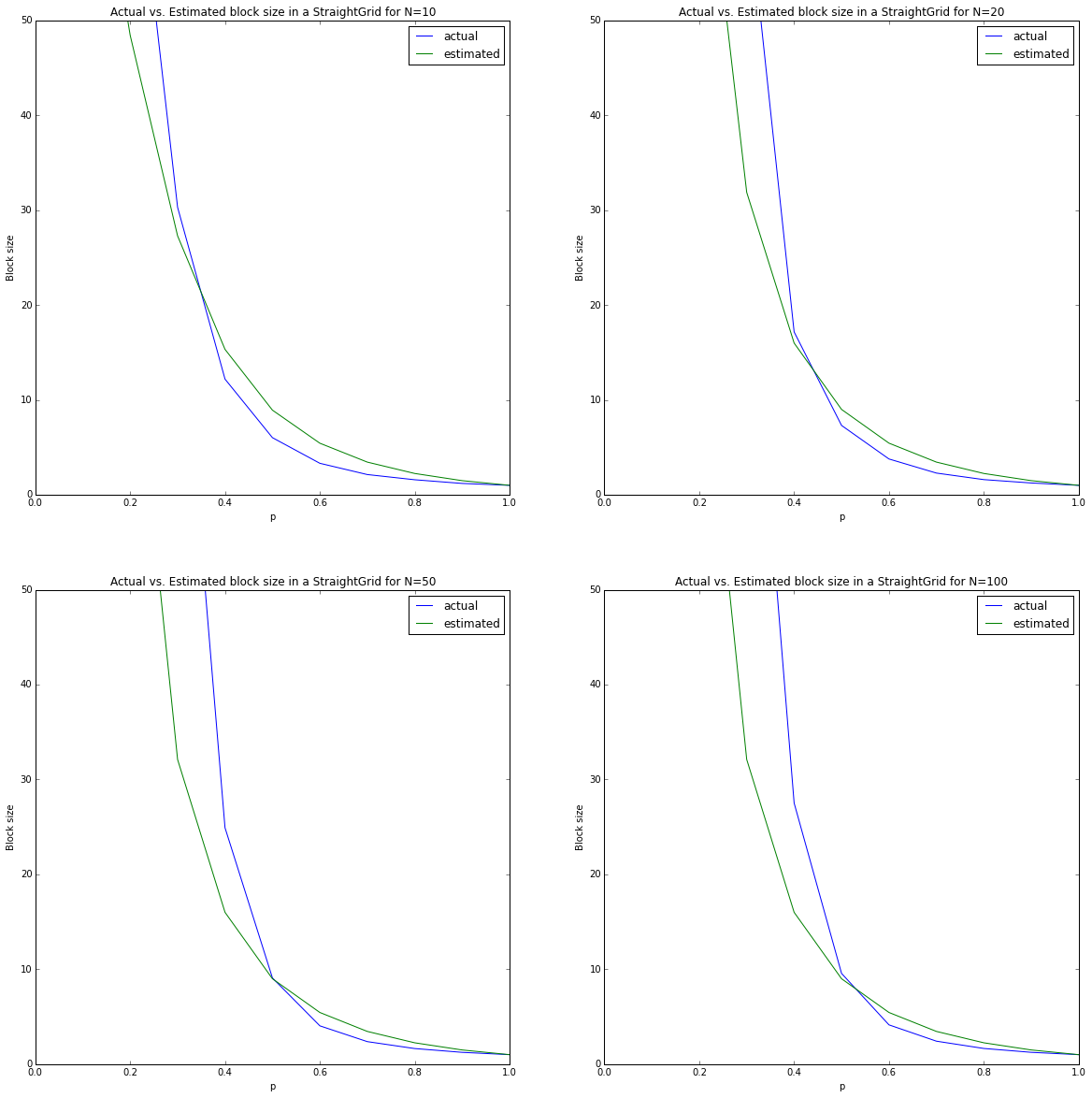
Performance of the Grid Expression
Here, I plotted the actual average block size (on 20 iterations) and the estimated one for all p’s and several N’s. From the previous section, we could already expect that the estimated block size won’t change much between N’s but here we can see that the actual block size also stays pretty constant.
As we’ve said before, the second assumption we’ve made (about the block’s shape) doesn’t hold in reality. We can clearly see it now with the much higher error than in the cyclic assumption we’ve tested before. It’s also clear that the error is not random over p. We should therefore suspect that this is an error due to bias in the model and not variance. That makes sense. We’ve limited our model to make it simpler. The price to pay now is that the estimation isn’t accurate, but again - we’re not trying to get to a 100% mathematical proof but to solve a problem we had, and for that - I believe this expression is enough.
By the way, if you’re interested in some more explanation on Bias vs. Variance in models, Prof Abu-Mustafa (CalTech) has an excellent course and covers this topic as well. You can find the lectures here. Lecture #8. But do yourselves a favor and watch all of them.
Summary
That was a long and a complex post and I found myself thinking about this problem for a few weekends now. Just thinking that I actually started from a completely different problem and expect this to be a 50 lines of code makes me think I should probably be more careful with my time estimations going forward..
If you got all the way here (and opened all math sections) - You’re da man!