
If you’ve ever worked with Spark on any kind of time-series analysis, you probably got to the point where you need to join two DataFrames based on time difference between timestamp fields.
For the purpose of this post, let’s assume we have a DataFrame with events data, and another one with measurements (couldn’t be more generic than that…). Both have timestamp fields (eventTime and measurementTime), and we want to join every event with the measurements that were recorded in the hour before it.
A naive approach (just specifying this as the range condition) would result in a full cartesian product and a filter that enforces the condition (tested using Spark 2.0). This has a horrible effect on performance, especially if DataFrames are more than a few hundred thousands records.
While Spark guys are working on a more generic solution (see github issue here), there are still use-cases we can greatly improve performance even with the current join strategies that are available. One of them is the one described above (events to measurements from the hour before it), and I believe it’s a very common one. In this post I’ll briefly go over the suggested implementation that worked for me, and if your use-case is different, you could probably play with that a bit so it addresses yours too.
The Data
To keep everything simple, we’ll work with the following dataframes. You can obviously work with your own classes as long as they have a timestamp or a numeric field. This example will use timestamps.
Events
root
 |-- eid: long (nullable = false)
 |-- eventTime: timestamp (nullable = true)
 |-- eventType: string (nullable = true)
Random Events can be generated using the following code:
case class Event(eid:Long, eventTime:java.sql.Timestamp, eventType:String)

val randomEventTypeUDF = udf(() => List("LoginEvent", "PurchaseEvent", "DetailsUpdateEvent")(Random.nextInt(3)))

def generateEvents(n:Long):Dataset[Event] = {
    val events = sqlContext.range(0,n).select(
        col("id").as("eid"),
        // eventTime is just being set to an event every 10 seconds.
        (unix_timestamp(current_timestamp()) - lit(10)*col("id")).cast(TimestampType).as("eventTime"),
        randomEventTypeUDF().as("eventType")
    ).as[Event]

    events
}

generateEvents(5).toDF.show

//   +---+--------------------+------------------+
//   |eid|           eventTime|         eventType|
//   +---+--------------------+------------------+
//   |  0|2016-09-12 15:46:...|     PurchaseEvent|
//   |  1|2016-09-12 15:46:...|DetailsUpdateEvent|
//   |  2|2016-09-12 15:46:...|DetailsUpdateEvent|
//   |  3|2016-09-12 15:45:...|DetailsUpdateEvent|
//   |  4|2016-09-12 15:45:...|        LoginEvent|
//   +---+--------------------+------------------+
Measurements
root
 |-- mid: long (nullable = false)
 |-- measurementTime: timestamp (nullable = true)
 |-- value: double (nullable = false)
Similarly, Measurements can be faked using this code:
case class Measurement(mid:Long, measurementTime:java.sql.Timestamp, value:Double)

def generateMeasurements(n:Long):Dataset[Measurement] = {
    val measurements = sqlContext.range(0,n).select(
        col("id").as("mid"),
        // measurementTime is more random, but generally every 10 seconds
        (unix_timestamp(current_timestamp()) - lit(10)*col("id") + lit(5)*rand()).cast(TimestampType).as("measurementTime"),
        rand(10).as("value")
    ).as[Measurement]

    measurements
}

generateMeasurements(5).toDF.show

//   +---+--------------------+-------------------+
//   |mid|     measurementTime|              value|
//   +---+--------------------+-------------------+
//   |  0|2016-09-12 15:46:..|0.41371264720975787|
//   |  1|2016-09-12 15:46:...| 0.1982919638208397|
//   |  2|2016-09-12 15:46:..|0.12030715258495939|
//   |  3|2016-09-12 15:46:..|0.44292918521277047|
//   |  4|2016-09-12 15:45:...| 0.8898784253886249|
//   +---+--------------------+-------------------+
The Naive Approach
If we choose to just join the DataFrames and specify the range condition, we’d get the following:
import org.apache.spark.unsafe.types.CalendarInterval

var events = generateEvents(1000000)
var measurements = generateMeasurements(1000000)

// An example with a timestamp field would look like this:
val res = events.join(measurements,
   (measurements("measurementTime") > events("eventTime") - CalendarInterval.fromString("interval 30 seconds") ) &&
   (measurements("measurementTime") <= events("eventTime"))
)

// With a numeric field (took the id as an example, this is obviously useless):
val res = events.join(measurements,
    (measurements("mid") > events("eid") - lit(2)) &&
    (measurements("mid") <= events("eid"))
)

res.explain

// run something like `res.count` to make Spark actually perform the join.
The important thing to look on, is how Spark plans to perform the join we’ve defined on our two DataFrames. The explain command, both on a timestamp field join, and on a numeric field join, gives us this:
== Physical Plan ==
CartesianProduct ((measurementTime#178 > eventTime#162 - interval 30 seconds) && (measurementTime#178 <= eventTime#162))
:- *Project [id#156L AS eid#161L, cast((1474876784 - (10 * id#156L)) as timestamp) AS eventTime#162, UDF() AS eventType#163]
:  +- *Range (0, 1000000, splits=4)
+- *Filter isnotnull(measurementTime#178)
   +- *Project [id#172L AS mid#177L, cast((cast((1474876784 - (10 * id#172L)) as double) + (5.0 * rand(6122355864398157384))) as timestamp) AS measurementTime#178, rand(10) AS value#179]
      +- *Range (0, 1000000, splits=4)
The first row is the key, indicating that Spark is going to resolve our request by performing a cartesian product of the two DataFrames. Notice that if number of records in one of the DataFrames is small enough, Spark will be able to broadcast one of them to all machines and perform a BroadcastNestedLoopJoin and BroadcastExchange. This is better, but isn’t considered as a solution as we want to work with large data sets.
The Bucketing, Double-Joining and Filtering Approach
Now let’s take advantage of our less generic use-case. We know that we’re only interested in measurements that happened up to 60 minutes before the event so basically, every event should only be matched with it’s local environment (time based) and a full cartesian product is just a waste of computing effort. We would basically like to group records together and join only groups of records that are close in time.
Let’s start with grouping records in both DataFrames by a 60 minutes interval:
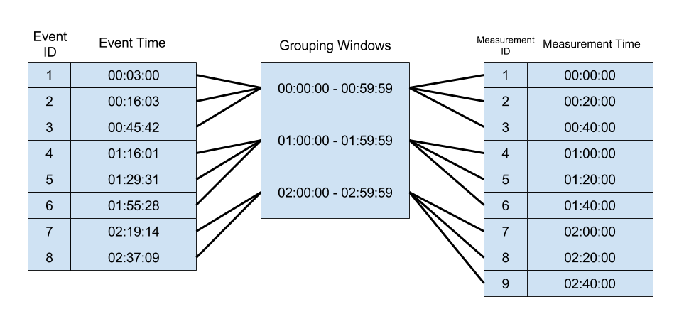
If we look on a specific event record, no matter where it’s ‘located’ in its timeframe window (the first minute or the last minute of the 60 minutes window), we can guarantee that all its matching measurements will either be linked to the same window, or the one before:
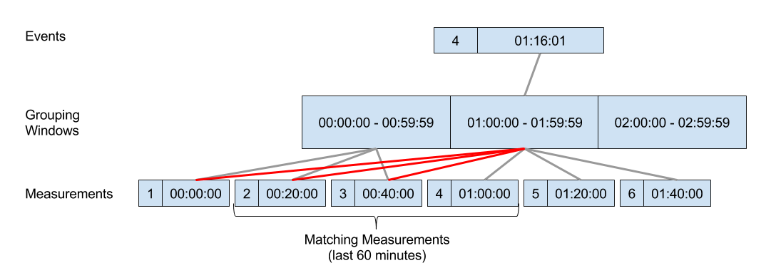
What we basically want to do is to group all events to timeframes, and link every measurement to its matching window and the one after (marked in red). Then, we can join by the window column and filter for the exact 60 minutes before (as the two frames will give us more than that). The same technique can be applied to numeric fields as well (grouping to windows is actually integer division). The following code does that for both cases:
import scala.util.{ Try, Success, Failure }

def range_join_dfs[U,V](df1:DataFrame, rangeField1:Column, df2:DataFrame, rangeField2:Column, rangeBack:Any):Try[DataFrame] = {
    // check that both fields are from the same (and the correct) type
    (df1.schema(rangeField1.toString).dataType, df2.schema(rangeField2.toString).dataType, rangeBack) match {
        case (x1: TimestampType, x2: TimestampType, rb:String) => true
        case (x1: NumericType, x2: NumericType, rb:Number) => true
        case _ => return Failure(new IllegalArgumentException("rangeField1 and rangeField2 must both be either numeric or timestamps. If they are timestamps, rangeBack must be a string, if numerics, rangeBack must be numeric"))
    }

    // returns the "window grouping" function for timestamp/numeric.
    // Timestamps will return the start of the grouping window
    // Numeric will do integers division
    def getWindowStartFunction(df:DataFrame, field:Column) = {
        df.schema(field.toString).dataType match {
            case d: TimestampType => window(field, rangeBack.asInstanceOf[String])("start")
            case d: NumericType => floor(field / lit(rangeBack))
            case _ => throw new IllegalArgumentException("field must be either of NumericType or TimestampType")
        }
    }

    // returns the difference between windows and a numeric representation of "rangeBack"
    // if rangeBack is numeric - the window diff is 1 and the numeric representation is rangeBack itself
    // if it's timestamp - the CalendarInterval can be used for both jumping between windows and filtering at the end
    def getPrevWindowDiffAndRangeBackNumeric(rangeBack:Any) = rangeBack match {
        case rb:Number => (1, rangeBack)
        case rb:String => {
            val interval = rb match {
                case rb if rb.startsWith("interval") => org.apache.spark.unsafe.types.CalendarInterval.fromString(rb)
                case _ => org.apache.spark.unsafe.types.CalendarInterval.fromString("interval " + rb)
            }
            //( interval.months * (60*60*24*31) ) + ( interval.microseconds / 1000000 )
            (interval, interval)
        }
        case _ => throw new IllegalArgumentException("rangeBack must be either of NumericType or TimestampType")
    }


    // get windowstart functions for rangeField1 and rangeField2
    val rf1WindowStart = getWindowStartFunction(df1, rangeField1)
    val rf2WindowStart = getWindowStartFunction(df2, rangeField2)
    val (prevWindowDiff, rangeBackNumeric) = getPrevWindowDiffAndRangeBackNumeric(rangeBack)


    // actual joining logic starts here
    val windowedDf1 = df1.withColumn("windowStart", rf1WindowStart)
    val windowedDf2 = df2.withColumn("windowStart", rf2WindowStart)
        .union( df2.withColumn("windowStart", rf2WindowStart + lit(prevWindowDiff)) )

    val res = windowedDf1.join(windowedDf2, "windowStart")
          .filter( (rangeField2 > rangeField1-lit(rangeBackNumeric)) && (rangeField2 <= rangeField1) )
          .drop(windowedDf1("windowStart"))
          .drop(windowedDf2("windowStart"))

    Success(res)
}
As you can see, most of it is just the handling of both timestamps and numerics. The logic itself is pretty straight-forward..
Let’s look at the execution plan now:
var events = generateEvents(10000000).toDF
var measurements = generateMeasurements(10000000).toDF

// you can either join by timestamp fields
var res = range_join_dfs(events, events("eventTime"), measurements, measurements("measurementTime"), "60 minutes")
// or by numeric fields (again, id was taken here just for the purpose of the example)
var res = range_join_dfs(events, events("eid"), measurements, measurements("mid"), 2)

res match {
    case Failure(ex) => print(ex)
    case Success(df) => df.explain
}

// and run something like `res.count` to actually perform anything.
When we run this (with a relatively large DataFrame to avoid broadcasting optimizations) we get the following execution plan (some text was truncated to keep is readable…):
== Physical Plan ==
*Project [eid#1449L, eventTime#1450, eventType#1451, mid#1469L, measurementTime#1470, value#1471]
+- *SortMergeJoin [windowStart#1486], [windowStart#1494], Inner, ((measurementTime#1470 > eventTime#1450 - interval 30 seconds) && (measurementTime#1470 <= eventTime#1450))
   :- *Sort [windowStart#1486 ASC], false, 0
   :  +- Exchange hashpartitioning(windowStart#1486, 200)
   :     +- *Project [eid#1449L, eventTime#1450, eventType#1451, window#1492.start AS windowStart#1486]
   :        +- *Filter ((isnotnull(eventTime#1450) && (eventTime#1450 >= window#1492.start)) && (eventTime#1450 < window#1492.end))
   :           +- *Expand (...)
   :              +- *Project (...)
   :                 +- *Range (0, 10000000, splits=4)
   +- *Sort [windowStart#1494 ASC], false, 0
      +- Exchange hashpartitioning(windowStart#1494, 200)
         +- Union
            :- *Project [mid#1469L, measurementTime#1470, value#1471, window#1500.start AS windowStart#1494]
            :  +- *Filter (((isnotnull(measurementTime#1470) && (measurementTime#1470 >= window#1500.start)) && (measurementTime#1470 < window#1500.end)) && isnotnull(window#1500.start))
            :     +- *Expand (...)
            :        +- *Filter isnotnull(measurementTime#1470)
            :           +- *Project (...)
            :              +- *Range (0, 10000000, splits=4)
            +- *Project (...)
                  +- *Expand (...)
                     +- *Filter isnotnull(measurementTime#1470)
                        +- *Project (...)
                           +- *Range (0, 10000000, splits=4)
SortRangeJoin instead of CartesianProduct is the key here.
Some sanity check
Events dataframe contained 10 events (one every 10 seconds). Measurements dataframe also contained 10 measurements with around 10 seconds between them. Below is the result of the join for rangeBack="30 seconds" (rows were truncated):
| eid | eventTime | eventType | mid | measurementTime | value |
|---|---|---|---|---|---|
| 3 | 18:24:28 | LoginEvent | 6 | 18:24:02 | 0.12131363910425985 |
| 3 | 18:24:28 | LoginEvent | 5 | 18:24:09 | 0.12030715258495939 |
| 3 | 18:24:28 | LoginEvent | 4 | 18:24:21 | 0.7604318153406678 |
| 4 | 18:24:18 | LoginEvent | 7 | 18:23:52 | 0.6037143578435027 |
| 4 | 18:24:18 | LoginEvent | 6 | 18:24:02 | 0.12131363910425985 |
| 4 | 18:24:18 | LoginEvent | 5 | 18:24:09 | 0.12030715258495939 |
| 5 | 18:24:08 | PurchaseEvent | 8 | 18:23:39 | 0.1435668838975337 |
| 5 | 18:24:08 | PurchaseEvent | 7 | 18:23:52 | 0.6037143578435027 |
| 5 | 18:24:08 | PurchaseEvent | 6 | 18:24:02 | 0.12131363910425985 |
| … | … | … | … | … | … |
Benchmarking
In order to estimate the performance boost, I launched a Google Dataproc cluster of 4 regular machines (plus a master) and tried different sizes of DataFrames. The results are below:
| Naive Approach | Efficient Approach | |||
|---|---|---|---|---|
| # Rows | Time (secs) | # Rows | Time (secs) | |
| 10K | 7.85 | 10K | 1.57 | |
| 20K | 7.81 | 50K | 2.48 | |
| 50K | 43.40 | 100K | 3.08 | |
| 80K | 97.73 | 500K | 14.09 | |
| 130K | 265.43 | 1M | 13.06 | |
| 200K | 736.58 | 2M | 17.49 | |
| 5M | 85.52 | |||
| 10M | 189.39 | |||
| 50M | 252.44 | |||
| 100M | 438.15 |
Results are pretty impressive. I could join dataframes with 50M records each at around the same time it took me to join 130K dataframes in the naive approach. I also tried to join larger dataframes with the naive approach but since I’m being billed by the minute, and it started to take hours, I just gave up…
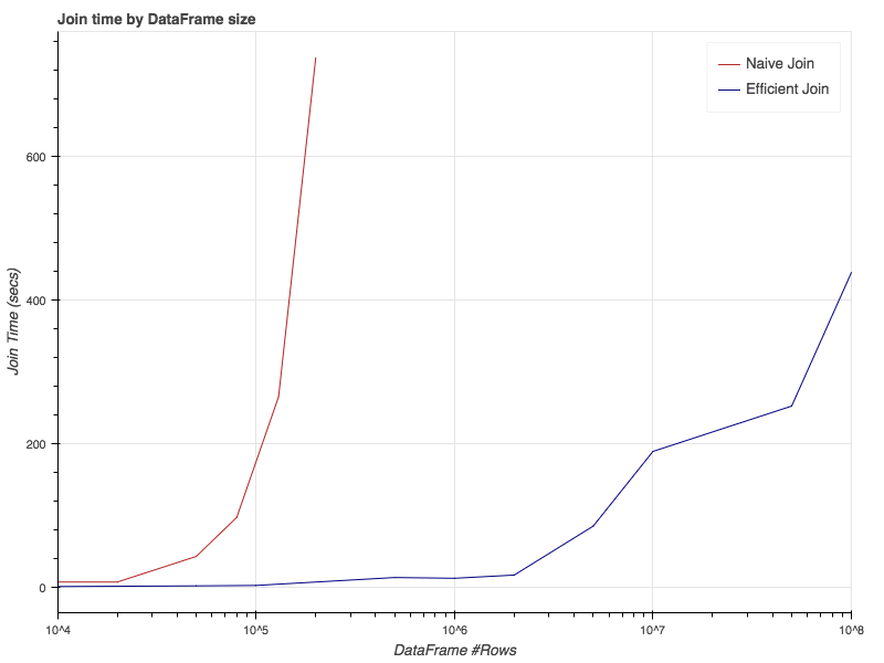
Notice the x-axis is logarithmic. The performance boost is actually around 3 orders of magnitude.
What if my use-case is different?
Well, depends on what exactly you mean by different. If instead of the last 60 minutes, you want to join anything from 120 to 60 minutes before the event, you could just play with the windows we attach measurements to. If you want to join to future measurements we’ll basically have to match measurements to past windows instead of the current and next one. All those changes are pretty easy to do.
If, however, you want to stretch the limits and try to join records where the rangeBack parameter isn’t constant (let’s say it depends on some field of the event), then you’re out of luck with this approach but I hope it at least gave you some ideas…
Hope that helps, and I actually really hope Spark devs will support range joins through Catalyst so we don’t need to hack our way to efficient joins.