
When life gives you GCP credits, make a Simpsons Detector!
I recently got one of those vouchers for GCP credits and started looking for a decent use for them before they follow their descendants in the expiration abyss. It just happened to be that I also watch the online Andrej Karpathy, Fei-Fei Li and Justin Johnson’s course (CS231n by Stanford) and thought that it might be nice to have my own final project like the ‘real’ students.
Last year I attended a data hackaton with some friends and our project for the weekend was trying to break Simpsons videos into sections and given a transcript from the user, compile them back to follow the script as much as we can.
When I thought about a final project for this course, I couldn’t resist re-using the Simpsons for image classification task. I trained a network to detect the four main Simpsons characters, allowing me to annotate a complete episode with a bar at the bottom that shows the currently visible characters.
It was nice, fun and took much more time and effort than I expected. I thought this post could be useful even if you are not a Simpsons fan (who isn’t??) as many of the concepts are very similar to other problems.
If you’re short on time, here is a highlights video. Enjoy!
Intro
This post briefly describes the work I’ve done on the Simpsons detector and goes over my main takeaways, insights and directions that worked best for me (and also those that were a complete waste of time…).
This is not intended to be a detailed intro to deep learning or convolutional neural networks but I’m happy to share some sources that helped me throughout the way. In general, knowledge in this area exists and for free, so help yourselves:
- CS231n - A (very good) Stanford class on image classification with deep learning. I think it’s excellent for people with general ML knowledge that want to dive deeper into DL.
Course notes (a great summary in general)
Lectures can be found on YouTube - Neural Networks and Deep Learning - A free online book by Michael Nielsen that goes over all main topics in DL while opening all the mathematical black boxes that sometimes remain closed.
- How Convolutional Neural Networks Work - Another nice post, with examples, on how convolutional layers work.
I’ve heavily used Jupyter Notebook as my main IDE. All notebooks are in my GitHub repo (GitHub has a nice renderer for ipynb files). I’ve also arranged some of the code into general and simpsons python packages and those are also available here. You are more than welcome to have a look although the whole post should be readable even without diving into the code.
Since the whole purpose is educational only, I wanted to use this exercise to demonstrate some concepts that are also useful in many cases in real life problems. Some of these make the problem harder to solve, and indeed, if it was a commercial project I might have considered a different approach.
-
Transfer Learning: We (the poor people without thousands of GPUs and endless amount of time and money) can’t afford to train large networks from scratch. One approach to solve this is by transferring the learning of another problem into our domain. I chose to use VGG16 trained network although it was trained on regular images (rather than cartoons) and apply those learnings into the Simpsons domain. It’s discussed with more details in this section.
-
Simulating Training Data: Sometimes we want to train our model on data that we just don’t have enough of (anyone says fraud prevention?). In these cases (and others), a common approach is to augment the training-set and generate many examples from the ones we have. This obviously adds the bias between our generated images and the real test ones as they don’t come from the same distribution anymore. It is an important point to keep an eye on and even allocate some of the test set to estimate this bias particularly. In this project, although I could just tag real frames, I wanted to learn from images that were freely available on Google Images and apply the learning on real frames. From my experience, it was the most time-consuming part of this project. This section deeply discusses that.
-
Human Performance: The end goal of this project is to detect the Simpsons characters as a human would do. For that I used HeatIntelligence’s service (similar to Mechanical Turk but easier to use) to submit real frames from Simpsons episodes to real humans and ask them to tag the characters that are in the frame. The following section explain some of the issues when dealing with human tagging.
I used Keras and Tensorflow to train and run my neural network and as I mentioned in the beginning, I had some GCP credits to spare so I was quite happy with the recent announcement about GPU general availability. I used a single NVIDIA K80 accelerator which costed me about 0.70$/hr. Unfortunately, GPUs don’t work with preemptible machines, that pushed the total prices higher. The extra rate was justified in my case as performance boost was enormous.
As a nice application to the model, I created a small tool that takes a video, detects which characters appears in it (frame by frame) and generates a video with a small bar of characters indicators on the bottom.
Diving into the Data
Generally speaking, I’ve used two different data sets: a training set of neutral characters images (not crops from real frames) and a test set of real frames from episodes. The training images were divided to train and train-dev (75%-25%) so I could make sure the learning process actually learns something and that I’m not overfitting. The test images were divided to dev and test (50%-50%) because we also have to make sure our frames generator is generalizing well and allows us to detect also real frames. The test set was only used at the end to estimate the final performance.
Generally speaking, with regards to data splitting, I followed Andrew NG’s lecture from the ‘Bay Area Deep Learning School’ - Nuts and Bolts of Applying Deep Learning. Kevin Zakka was kind enough to summarize it in his blog if you prefer the textual version.
Originally I wanted to include Maggie too, but couldn’t find a large enough training set for her (only around ~15 images). Because she looks a lot like Lisa it hurt both characters performance and I decided to just drop her.
Train & Train-dev sets
As was mentioned before, one of the key points of this exercise was to demonstrate learning from a training set that came from a different distribution than the test set. This is a fancy way to say - I’m not going to train on real frames but on other images that I’m going to make look like real frames. The obvious advantage here is that I can generate as many samples as I want. The drawback is that my generated frames will probably not be exactly as the real ones, hence, there is a risk of learning features that are unique to my generation process and won’t generalize well to real frames.
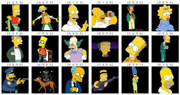
I trained the network using ‘neutral’ images I found on Google Images. I had a script that downloaded the search results and I manually filtered out all kind of weird stuff you get when you search for “Bart Simpson” and is not really Bart Simpson… Since I wanted to stitch a few images together, I chose only images that were on a clear background (white, black or any solid color that I could easily take out later).
I run this script for every character I could think of (including Maggie, Apu, Krusty, Milhouse and many more). That got me ~900 images. Getting examples of ‘other’ characters is important as otherwise, the network would have probably learned that the yellow color is always correlated with a positive prediction and I wanted to make sure it learns more specific features for every character.
Background was cropped from all images and every image was rescaled to 300x300 pixels. This will allow me to rescale later when I generate a ‘real’ training frame without losing much quality.
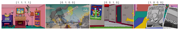
Training images were tagged with a one-hot encoded vector that could also be a vector of zeros in case the character is not one of the major four. Characters order in the vector is: [Bart, Homer, Lisa, Marge].
Here are some examples of training images. As you can see, separating the image from the background is not always perfect (e.g. Apu in the 1st row), and sometimes, all image manipulation algorithms can ruin the image (e.g. Marge’s eyes in the 3rd row were cut as a part of the background). I worked quite a lot to get to something that works nicely on most of the cases, and although I could manually remove those images from the training set, I didn’t do it as life isn’t perfect and every training set will have some errors or faulty data points.
Test & Dev sets
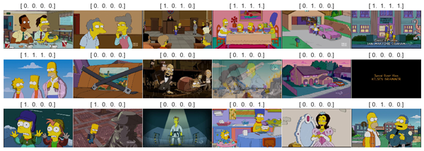
In order to evaluate the performance of my model, I extracted ~700 frames from ~100 random Simpsons videos. Videos are 720p so every frame is 720x404 pixels (RGB) and frame rate is 24fps.
I actually started with much less episodes (around 5), but randomly got an episode where Bart and Homer went to a baseball match and Bart was wearing a baseball cap for half the episode. That obviously degraded performance, as even before I discuss the network in more details, you could expect it to identify Bart’s unique hair shape which did not exist in this episode almost at all.
When I analyzed the results after the first couple of runs, I saw the bias and fixed it by sampling fewer frames from many episodes.
I divided the 700 frames equally between test and dev sets. Both are real frames, but their purposes are different. dev is used to validate that we can apply the learning of the model (that was trained on train) on real frames and to calibrate some decision thresholds (set a specific recall or maximize accuracy for example after a model was trained). The test set was only used once, at the end, to get final performance metrics (which weren’t different from what was measured on dev).
Test images were manually tagged with HeatIntelligence’s API. You can easily create requests for manual intervention in your flow and collect the responses. I’ve used their API to create a request with an image and 4 checkboxes that the agent would tick to indicate that a specific character appeared in the image. Costed my around ~15$ to tag ~700 frames and was very quick (a couple of minutes)!
Below are some examples of test images:
Generating Simpsons Frames
Data scientists like to say that 80% of every project has nothing to do with models, networks and other fancy stuff and is only about a painfully, rigorous work of obtaining and cleaning the data. In a similar way, I can admit that looking back, more than 95% of my time was spent on improving the frames generator and not the network architecture. The frames generator was also proven to be responsible for all performance boosts I had throughout this journey. Almost every time I improved the way I stitch images together, the augmentations I do to images or background choosing, I immediately saw the affect on performance.
The generator is implemented in the SimpsonsFrameGenerator class and complies with Keras’s generators API. it returns an iterator that yields a batch of X and y every time next() is called on it. Every single frame is generated as follows (high-level, a more detailed description will follow):
- Choose a random background
- Choose the number of characters we want to add to the frame (could also be 0)
- Choose the actual training images we’ll use
- For every image - randomly play with horizontal-flipping, scaling and rotation
- Stitch all images on the background
As with everything, god is in the details. I had to spent quite a lot of time to make stitching better, to better place many images on a background while minimizing overlapping and many other tiny pain-points, but at the end, this is what my generator produces:
Frames Backgrounds
Since we want to simulate a real frame, and not just a bunch of characters on a black background, we’ll need to start with a ‘neutral’ background and stitch characters on it. My problem was how to efficiently find candidates for background images.
I ended up with a heuristic that worked pretty well and didn’t require any manual work. I started with a couple of episodes (other than the ones I’ve used for testing) and extracted some frames from them.
Then, in order to filter out all frames that contained a character I scored every frame by the amount of ‘Simpsons-yellow’ that appears in the frame. ‘Simpsons-yellow’ is [255,217,15] in RGB and I counted every pixel that was close enough to this value. I required every background image to have less than 1% of simpsons-yellow and less than 75% of black (to avoid the credits at the end).
That gave me around 200 images, which I thought is enough. Like with all my previous automatic stages, there are some errors (Homer appears in the 4th row twice where he shouldn’t have been), but generally speaking that was satisfiable and didn’t require any manual tagging (meaning - easily scalable in case I neede to). Some examples are below:
Frame generation
When generating the frame, there are two main choices we have to make. The first is simple and is just choosing a random background from the ones we’ve generated before. The second is choosing which images from the training set we’ll put on top.
Like everything else in the process, I didn’t have any idea on what the winning strategy would be, I implemented everything as generic as I could through many hyper-parameters that I tuned later. I used the following hyper-parameters for the frame generation process:
- Maximal number of characters in the frame: every frame will randomly choose a number between 0 and this parameter (inclusive).
- Number of characters probabilities: if given, use to skew the choosing of num_characters. Otherwise uniform sampling is used.
When we know how many characters we want to add, we choose (without replacement) from all available characters in the training-set (the four main ones plus ‘others’). Last stage is to choose the actual image we’ll use for every character. This is also chosen randomly from the training set for every character we need.
To allow even more variations in the training images, I’ve used the Keras ImageDataGenerator to flip and rotate the image, and I’ve implemented my own scaling that deals with transparency better. All three are also hyper-parameters which I’ve played with to get the required results and ended up with:
- Horizontal-flipping: allowed
- Rotating: up to 20° both sides.
- Scaling: between 25% and 85% of the original image (training images are 300x300, generated frame is 202x360).
Transfer Learning
Transfer learning refers to using a network that was previously trained by someone else and apply the learned features to our problem domain. The motivation to do so is mainly to take advantage of others with a lot of data and a lot of resources who have already trained a network to deal with a similar problem.
There are a lot of work around image classification with deep learning, and many networks were trained by the best researchers in the world who have access to tons of GPUs. Most of the networks are trained on a dataset called ImageNet. ImageNet is a dataset of ~1M images from 1000 categories and people are competing who will train a network that outperforms the others. As everything else in this area, it’s very common to open-source the model architecture and weights.
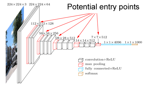
I chose to start with a network called VGG16. It was created by K. Simonyan and A. Zisserman from the University of Oxford and achieved 92.5% top-5 accuracy on the ImageNet challenge. Newer networks tend to be either more complex or very deep and that might have added some challenges while I’m trying to integrate it into my model. VGG is a classical bunch of convolutional layers combined with a few fully-connected ones and an output layer. This makes it pretty straight-forward for me to hook into one of the convolutional layers and add my own fully-connected layers on top to learn the specific Simpsons features.
A major concern was that all commonly used pre-trained network (and VGG among them) were trained on a set of ‘real’ images. I was going to use it as a base level to detect features in a cartoon image which looks very different from a camera image. Even without being an image classification expert, I could expect colors, object edges, shades and almost every other aspect of the image to be different. Since I couldn’t find any other network that was trained specifically on cartoons, I started with VGG and eventually this concern wasn’t a real problem.
Generally speaking, the network itself that I’m transfer learning from (VGG in my case), and the exact ‘entry-point’ (5th conv layer in my case) are hyper-parameters to the model. While I didn’t bother to try various networks (mainly because it might cause an architectural change), I did play with the entry-point and tried the weights after every one of the 5 convolutional layers in VGG. Results were very clear that learning is best when I use all 5 layers so I quickly fixed this parameter and moved on.
Network structure
Building the network is again a game of many hyper-parameters. I wrote the create_model function to be as generic as I could, and played with various combinations of those parameters to see what works best.
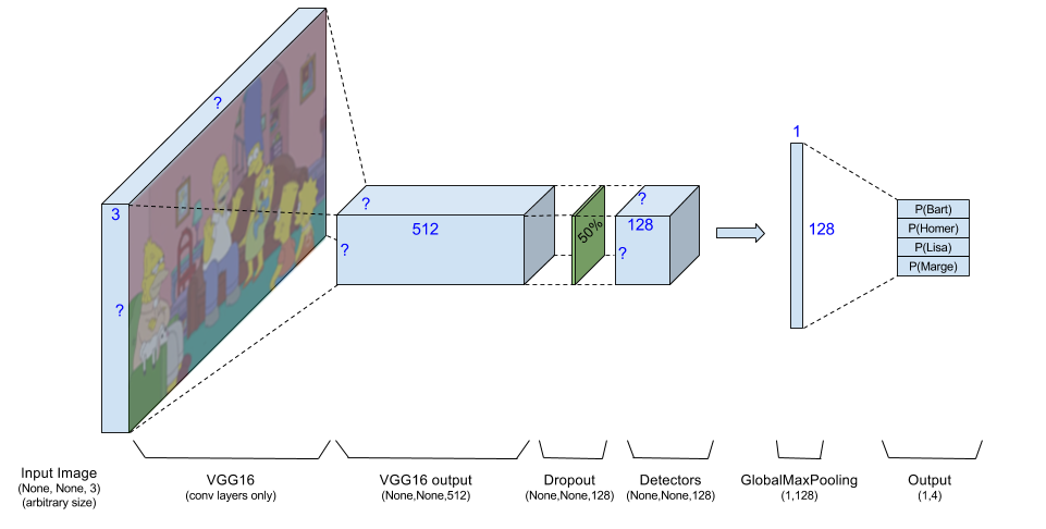
My network starts with an RGB image. Theoretically, the network accepts an image of arbitrary size (annotated in Keras as [None,None,3]), but practically I always feed it with 202x360x3 images. This image goes through VGG16 which outputs the activation maps of 512 neurons. I use the VGG output as an input to the rest of the network.
I optionally add a batch-normalization layer on the VGG output. Eventually I decided not to use it as it degraded the performance on the test-set and I must admit I didn’t expect that. BatchNorm is a ‘meta-layer’ added to the model at specific points to reduce the Internal Covariance Shift. I won’t get into details, you can read that in their paper, but while I could expect it to slow the learning process a bit, my intuition was that it will actually help performance to scale all VGG outputs right before we start messing with them. I was wrong, and abandoned this option, but it’s still optional in the code.
Dropout is used right after VGG as a common measure to prevent overfitting. I played with various values for the dropout ratio and ended up (quite as expected) with the ‘regular’ 50%.
Next is the main part of the model, which are the detectors. After playing with it, I’ve used 128 detectors but this is obviously a hyper-parameter. Every detector is a linear combination of VGG outputs (still working on the activation maps so locality matters), and after having 128 activation maps I reduce every one of them to it’s max value. If we try to imagine what is each neuron’s role, then a specific detector might activate when it sees Bart’s hair (that means that somewhere in it’s activation map there will be a point with a high score). I’m not interested in the position of Bart in the image, so I only take the maximal activation for every detector.
Detectors (before the GlobalMaxPooling) are implemented as a convolutional layer of size 1x1 which keeps the activation map the same size and only allows linear combinations of neurons in the same place from different VGG outputs. After the GlobalMaxPooling is applied, every activation map is reduced to a single value, hence we have a vector of num_detectors values. Detectors are also implemented with a L2 regularizer on weights, regularization value is also controlled by a parameter.
I must say that I also tried to have several linear combinations before getting to the final 128 detectors (i.e. 512->256->128), and although that didn’t seem to help, if I had more time/money this is something I would try again. The fc_detectors parameter (fc for fully-connected) controls that.
The last layer is a fully connected layer that takes the 128 detector outputs into a vector of size 4 with the sigmoid activation function to generate values between 0 and 1.
The model is trained with adam as the optimizer (also a parameter), and MSE (mean squared errors) loss function so every output is practically a separate classifier with the same affect on the final loss. This also allows removing/adding characters as required.
As a last step, I also allowed re-training of VGG’s parameter (also known as fine-tuning). Both for performance reasons and because it didn’t prove itself as a beneficial idea, I’m not using this in the final model.
To summarize, hyper-parameters for building the model and the values I’ve used are:
- base_output_layer: ‘block5_pool’ (entry-point on VGG16)
- num_detectors: 128
- fc_detectors: [] (practically disabled)
- batchnorm: False
- dropout: 0.5
- reg_penalty: 0.001 (L2 regularization value for the detectors weights)
Human Performance
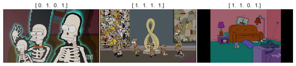
As mentioned before, I used humans only to tag the test frames (which will be used to evaluate performance) and after getting the tagging results back I noticed that human performance is ‘too good’ and sometimes involves ‘knowledge’ that I don’t expect the machine to have. I brought some representative cases just to show how difficult can it be to achieve 100% detection. You can also see that out of ~700 test images, I could easily bring around 20 images where I can’t expect the model to behave as good as a human. There were many more…
Because it didn’t seem as negligible at all, I wanted to get a ‘real’ feeling of how good the classifier is. I went over random 100 tagged images and marked how many times I ‘agree’ that the human tagging is something that I would expect from the model. Results were pretty consistent on all characters and were around 85% ‘expected recall’. That means I expect the model only to get to a recall of 85%. The other 15% are beyond automatic detection in my opinion, at least at this stage. The ‘expected recall’ helped me later as a guideline when I tried to set thresholds on the model predictions.
I train the network on nice face-forward images, and although I rescale every image to get to very small and very large characters, I obviously don’t cover all cases. The following examples show images where the characters appeared either very small, from the back, having a different hair-style or in different colors than expected (the labels are the human tagging):
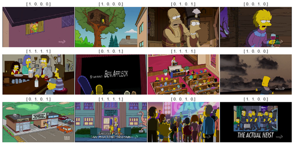
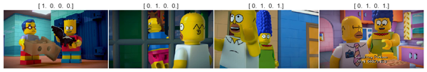
Next ones came from an episode where they all appear as Lego characters. An obvious un-predictable one:
The following are just some other weird cases. You can see that at the first image, the agent tagged all of them because they appear in the picture on the wall. In the second one, Homer is faded out. The third contains just enough of Lisa for a human to detect and the forth has Bart, but gray-scaled, inside a picture and with something on his eyes:
The last group of examples are what I call ‘human knowledge’. We have some additional knowledge about the show itself and the world, so we can extrapolate even when not everything is seen in the image. For example, the X-Ray doesn’t look like anything the network has seen before. We, as humans, know what an X-Ray is, so it’s easy for us to understand that these are Homer, Marge and Maggie. In the second image, we can only see the general shape of all the five characters. That alone, with the fact that we can somehow expect to see the whole family together is enough for us to know that they are all in the image. We also know that at the beginning of every episode they all sit on the couch, so in the last image, given Homer’s (?) leg and Marge’s hair, we conclude they appear in the frame. (I have no idea why the agent also tagged Bart…)
Setting Classifier Thresholds
After the model was trained, I could feed it with a batch of images and get predictions. Those vectors of predictions are between 0.0 and 1.0 and in order to clearly cut it, I had to set a threshold. Like with any binary-classification problem (this model is actually 4 binary-classifiers running together), we can set the threshold to achieve different values for precision and recall.
Not like in a real-world problem, I didn’t have any tangible loss function here. I’m not losing money if I predict wrong and I’m not in some kind of a competition where someone else defines the score (which I want to maximize). I only wanted something that looks nice to a human.
I generated 4 different boolean results from the same model predictions. One was set to achieve a recall of 75% (which is pretty high considering that 85% was the ‘maximal expected recall’ as was mentioned before), the second achieved 75% precision, the third was set to maximize the f-score and the last maximizes the accuracy.
I then just browsed through the results and chose the f-score as the one whose mistakes were the most ‘understandable’ for me and these were the thresholds I’ve used for predictions.
After optimizing for f-score, I run a report with accuracy and a confusion matrix for every character. The full results can be seen in the notebooks. I only copied the accuracy values:
| Character | Accuracy (%) |
|---|---|
| Bart | 86.3% |
| Homer | 74.4% |
| Lisa | 88.9% |
| Marge | 91.7% |
Video Tagging
When the model was ready, it was finally the time for the fun part - building a real application around it. Since prediction time on regular CPUs isn’t something I’d let users to wait, I created a tool that receives a video as input, tag it (currently set to extract 4 frames per second for tagging) and rebuild another video with a bottom row of indicators that are gray-scaled and get colored when their character is predicted to be in the frame. A picture is worth a thousand words:

All video extracting, concatenation and placement were done with MoviePy. After a short learning curve, you’ll be pretty impressed how easily you can do things like what I did (took me one night of coding, most of it on placement issues).
Predictions Smoothening
Although video tagging sounds like a purely technical issue, there is something to notice there. The model was trained on single images, without the context of a video (for example - what frame was before the current one). This is obviously something that will affect the prediction as if Bart was in a specific frame, he is most likely to appear in the next one too.
The more classical deep-learning approach to embed the knowledge from a sequence of images into the learning process would be using some kind of Recurrent Neural Networks. For the sake of my sanity I kept the model simple, having it digesting one frame at a time, but since there is some additional information in a sequence of predictions, I applied a simple heuristic to smoothen the results.
I scanned the predictions for the whole movie, character by character, in a rolling window of 5 predictions at a time, and if I could find a sequence of 5 predictions where there is only one ‘outlier’ and it is not in one of the edges, I’d override it. For example: [0,1,0,0,0] => [0,0,0,0,0] and [1,1,1,0,1] => [1,1,1,1,1].
This helped with some cases of single-frame glitches. It can’t help when the model doesn’t see the character in general (when it’s from the back, looks weird, or just a regular false-negative).
Video Examples
Copyright regulations prevent me from uploading full episodes so I’ve created a highlights video (embedded on top) with some examples of nice predictions and common mistakes. Most of it was already discussed in the previous sections. The video highlights just go over the main model weaknesses I’ve described and also some nice catches.
Takeaways
This has been a long road from the moment of “Yeah, should be pretty easy to detect the Simpsons, it’s only four cartoon characters” (Z. Moshe) to having a trained model and a finished post about it. I wanted to share some of my takeaways from this project. I believe they are common to this field and would help anyone who is trying to tackle a similar problem.
-
Take Small Steps: I mean really small. There were dozens of times where I was going over the results of one of the models and had many ideas on how to make the frame generator better (I mentioned before that the frame generator was the most valuable component in terms of time-spent vs. performance-boost gained). Every time I tried to implement them all and launch a new training I’d get inconsistent results and couldn’t tell which of the changes was good and which didn’t give the expected boost. Besides, even if I could tell, many times I’d add a feature (controlled by some hyper-parameter), thinking that I know how to use it best, only to later find out that a different configuration gives better results. Fine-tuning parameters one-by-one and when all other are fixed is much easier.
-
Manual Gap Analysis: I did have all kind of statistical measurements to estimate the performance of my trained model, and I’m clearly not against a numeric metric, but sometimes just having a look on correct and wrong predictions immediately showed me what the next problem to tackle is (small characters, rotated characters, different lighting). If you work on a domain where you can see/read your output - do so!
-
Dump Your Thoughts Somewhere: I only started doing this in the middle of the project and quite sorry I didn’t start from the beginning. I maintained a log table for all training runs I did with the hyper-parameters values, performance and a free comments field. After a week or two I could barely remember what other ideas I had in mind before I implemented others, or what were the results when I tried with/without a specific parameter. I must admit though that a textual table like I used is not ideal. I wanted something that I can attach images to (learning rates and other performance charts for example) and that is more similar to a mind-map. I tried all common mindmaps/leadpools/notes apps but couldn’t find exactly what I was looking for…
Future ideas
This project is not done. There is always some room for improvement and if you have watched the highlights video you probably saw there are some scenes with harsh mistakes. Actually, the reason I stopped improving the model is partially because I’m getting sick of the Simpsons but mainly because I don’t have any GCP credits left…
Assuming I had more time and money, here are a list of things I’d want to try:
-
Localization: Although the final layer of the network discards the spatial information on the detectors (with the GlobalMaxPooling layer), we can always get the activation map for each neuron and find where (approximately) in the image the feature appeared. I super cool demonstration for that would be to make the whole frame gray-scaled and leave the colors only on the characters. Thanks Doron Kukliansky for the idea!
-
Training set generation vs. Real images: One of the main concepts I wanted to use here was to learn from training data that is not the same as the test one. It will be interesting to compare results of the same model when it is trained on generated data vs. real frames. I’ve used ~50K generated training images. Extracting frames from episodes is not a problem, and based on my rough calculation, with HeatIntelligence’s API it would cost around 750$ to tag 50K images. Not that much but I might find some better uses for 750$…
-
RNNs: As I mentioned before, another nice idea to try is to build a recurrent network that consumes the sequence of frames (the whole video) and generate smarter predictions.
-
Client-side application: I saw Andrej Karpathy’s work on ConvNetJS, a JS code that can run (simple) networks directly inside your browser. While the current model is too large for that (~50MB) and probably uses layers that are not implemented in ConvNetJS, it would be nice to see how much it can be shrunk without effecting performance and maybe even running in the browser.
-
Ensemble: When looking on results from many different models, I saw that the common errors are not always the same. Meaning, one model could confuse Maggie for Lisa, while another one wouldn’t detect small characters well. This leads to thinking of an ensemble of models as a solution. I didn’t have enough credits to completely re-train a couple of models so I decided to try some technique that was mentioned in one of the meetups I attended recently. The speaker (Gil Chamiel, Taboola) mentioned they have used a ‘pseudo-ensemble’ by running the same model a few times with the dropout layer enabled (like in training phase). They had a regression problem, and they used the ensemble to get a measure for the confidence in the score. I tried it to see if can help my problem, although theoretically speaking, I couldn’t see how it can improve the learning itself and indeed, it didn’t improve anything…