Recently, the TensorFlow team announced their public 2.0 beta API
and I thought that would make a perfect excuse to see what has changed (and
plenty should have changed from the 1.x API…).

Keras is now the recommended
high level API
and this post will focus on subclassing keras.Layer to implement our own model.
The model we’ll look at is a fairly simple one, but could be useful for some real
domains other than this demonstration.

Code is shared in a public GitHub
but it’s pretty short and we’ll go over all of it here. I’ve used this Colab
to play with the code and run the examples section (if you’re not familiar with Colab - watch this). Colab is by far my favorite
research and playground environment. Plus - they give you a free GPU! This and a
good cup of coffee will make me happy forever…

In order to keep this post focused, I’m not going to go over “what has changed in
TF2.0” but a lot has. You can find interesting overviews here,
here and here.

The Sum of Gaussians Model

The sum of gaussians model assumes that for every datapoint X, the value of y
is the sum of K gaussian functions, each with arbitrary mean, covariance matrix
and a multiplying factor (will be referred to as amplitude in this post).

(Notice that unlike in the normal distribution PDF case, this expression is
slightly different as it doesn’t integrate to one. We use an arbitrary weight \(a\)
for every gaussian).

Our data will consist of datapoints and their y value, and we’ll try to recover
the centers, covariance matrices and amplitudes of the K gaussians that were
originally used to construct the data.

A real life example

Imagine you work at the analytics department of Starbucks. You have geo-locations
of many (many) selling points that Starbucks has all around the US and you assume
that people are more likely to have coffee at a branch that is close to where they live.
You want to estimate where people live, based on number of customers visiting each store.
If we assume that people live in K major cities in the area, every city’s population
can be modeled as a gaussian centered at the city center. The covariance matrix will
represent how spread the city’s population is, and the amplitude represents
the number of people living there.

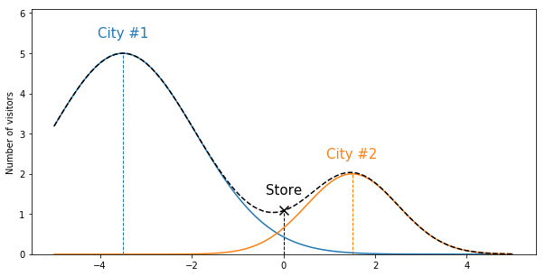
With this simplification of the world (and consumers’ behavior..), we can now say
that the number of customers that a specific store sees is the sum of the number
of visitors it got from each city. Let’s look at a 1D world:

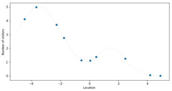
Now imagine you have many stores, but you only know the total number of visitors
and want to figure out where the cities are and how spread the population is. In
this example, training a SumOfGaussians model with 2 learned gaussians should
recover the centers (cities locations), covariance matrices (population spread in
each city) and the amplitudes (number of citizens per city).

Implementing a Keras.Layer

A Layer is a core component in Keras. It encapsulates a set of weights (some
could be trainable and some not) and the calculation of a forward-pass with inputs.
A Model in Keras is (in its most basic form)
a sequence of layers leading from the inputs to the final prediction.

In order to use a layer in a non-sequential
model we need to understand the difference between building a layer and invoking
it with inputs. When building a layer, we create Tensorflow variables for all
required weights. When we want to calculate our layer’s output, we call its
instance with the input tensors. This allows us to share weights between some
parts of the model (when using the same layer instance).

inputs = ...
my_dense = tf.keras.layers.Dense(10)  # Just creating the layer.
layer_output = my_dense(inputs)  # Invoking it and get a Tensor with the results.

other_inputs = ...
other_output = my_dense(other_inputs)  # Same weights will be used here.

When subclassing from keras.Layer
there are 3 important methods we need to understand:

• __init__(): We can initialize anything that doesn’t require the input’s
  shape here (we don’t have the inputs at this point). For example: general
  parameters, inner layers objects, etc…
• build(input_shape): Here we already know our input shape, therefore, we
  can create actual variables. For example, a Dense layer will create the kernel
  and bias variables here.
• call(inputs): This is where we define the forward pass of our calculation.

Implementing an initial version of SumOfGaussians

After we’ve mastered the keras.Layer API, let’s move on to implement a layer
that fits our sum of gaussians model. We’ll build the model for a known value of
K (this will be provided when constructing the layer). We need trainable variables
for the centers, covariance matrices and amplitudes. The forward pass is relatively
straight forward:

class SumOfGaussians(tf.keras.layers.Layer):
    def __init__(self, num_gaussians, **kwargs):
        super(SumOfGaussians, self).__init__(**kwargs)
        self.num_gaussians = num_gaussians

    def build(self, input_shape):
        self.dim = input_shape[-1]

        self.means = self.add_weight(
            'means', shape=(self.num_gaussians, self.dim), dtype=tf.float32)

        self.sigmas = self.add_weight(
            'sigmas', shape=(self.num_gaussians, self.dim, self.dim), dtype=tf.float32)

        self.amps = self.add_weight(
            'amps', shape=(self.num_gaussians,), dtype=tf.float32)

    def call(self, inputs, **kwargs):
        del kwargs  # unused.
        per_gaussian_output = [
            calculate_multivariate_gaussian(inputs, self.amps[i], self.means[i], self.sigmas[i])
            for i in range(self.num_gaussians)]
        result = tf.reduce_sum(tf.stack(per_gaussian_output, axis=-1), axis=-1, keepdims=True)
        return result

So far - nothing too complicated. We created the variables in the build() method and
generated the model’s output by summing the values from each gaussian. The
calculate_multivariate_gaussian method is just the expression for a single
gaussian function value given amplitude, mean, covariance and an input vector.
You can go over the implementation in GitHub.

Several problems with the naive implementation

Well.. Although it’s short and good for demonstration purposes, our naive
implementation doesn’t really work. I’ll go over the main problems, each will be
an opportunity to demonstrate another Keras way of doing things:

One can not just perform SGD on a covariance matrix

The sigmas variable is supposed to hold the covariance matrices for the K gaussians.
Every covariance matrix has to be positive semi-definite
and ours even has to be invertible. Our first problem hits us even before
running the first batch through our layer. Weights are initialized randomly by
default, meaning our sigmas variable contains random values and possibly not
PSD to begin with. We can solve this by overriding the initializer to use for
this weight.

For simplicity, let’s initialize all matrices to the identity matrix. An
initializer in Keras is a callable that receives the shape of the variable to
initialize and returns the value:

def _multiple_identity_matrices_initializer(shape, dtype=None):
    del dtype  # unused.
    assert len(shape) == 3 and shape[1] == shape[2], 'shape must be (N, D, D)'
    return np.stack([np.identity(shape[1]) for _ in range(shape[0])])

Then we can pass this one as the initializer of our weight:

class SumOfGaussians:
  def build():
    ...
    self.sigmas = self.add_weight(
      'sigmas', shape=(self.num_gaussians, self.dim, self.dim), dtype=tf.float32,
      initializer=_multiple_identity_matrices_initializer)

Looks like we’re safe for now, but what happens after the first SGD iteration?
If we recall how SGD works, we perform a forward pass through our network, get a
final value, calculate a loss based on the true value and calculate gradients on
the loss with respect to all weights. Then we modify the weights’ values based on
the computed gradients.

This means that even though our covariance matrix started with a valid value,
nothing assures us that it will remain valid after the back-propogation step.
In order to solve this, we’ll use a little trick - we’ll use the fact that every
matrix multiplied by its transpose is positive semi-definite.
Meaning, we can actually perform our SGD on a “pseudo_covariance” matrix, and when
we need the true covariance matrix for calculation, we can simply use
\( AA^T + \epsilon I\) (we’re also adding an identity matrix multiplied by a small factor to avoid singular
matrices).

Some minor changes are required for this change but they are mostly technical.
You’re welcome to take a look in the full implementation in GitHub.

Smarter initializers for the centers and amplitudes

Similar to the previous problem, we have some other problems with Keras’s defaults.
Our means will be initialized with glorot_uniform by default.
This returns values centered around zero with relatively small standard deviation.
This might work if the true centers are around zero, but if not, our model will
have a hard time trying to move the centers. Recall that if we’re too far away from
the gaussian center, its contribution to the sum is almost zero and the gradient’s
direction won’t lead us anywhere.

This is why we want to initialize the centers all around the practical input space.
Since we don’t know that in advance, we’ll allow the user to pass centers_min
and centers_max when constructing the layer. This will helps us initialize
the centers uniformly in that range.

class SumOfGaussians:
  def __init__(... centers_min, centers_max, ...):
    ...
    self.centers_min = np.array(centers_min)
    self.centers_max = np.array(centers_max)

  def build():
    ...
    self.centers_initializer = tf.keras.initializers.RandomUniform(
        minval=self.centers_min, maxval=self.centers_max)

    self.means = self.add_weight(
        'means', shape=(self.num_gaussians, self.dim), dtype=tf.float32,
        initializer=self.centers_initializer)
    ...

For the amplitudes we’ll be using a straight-forward vector of ones as an initial
value with the built-in tf.keras.initializers.Ones() initializer.

Analytical improvements

The following section will discuss a few additional improvements we can add.
These are not required technically, but are heuristics I’ve decided to add to
improve our chances to converge to an acceptable solution under “real-life”
conditions.

First, consider the fact that we might not know the real K when trying to converge
to a solution. For a visual and simple case, let’s assume our true data is sampled
from a single gaussian centered around 0.0, with a standard deviation
of 1.0 and an amplitude of 1.0, but we set K=2 in our model so we are going to
find a sum of 2 gaussians that fit this data.

One possible solution would be two gaussians that have the same center and
covariance matrix, and their amplitudes will sum up to 1.0 (Example #1).
Another solution could be two completely different gaussians which are summed up
to a gaussian very close to our original one (Example #2).

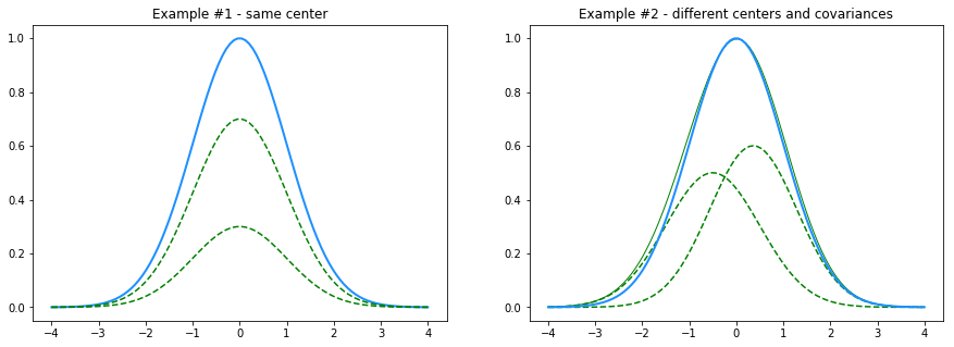
We’ll try to come up with heuristic solutions to these problems:

L1 regularizer on the amplitudes

I could guess that in a real-world scenario, if I overestimated K, I’d ideally
want excess gaussians to have an amplitude of 0.0 so I can easily exclude them from
my analysis. You can think of Example #1, when one of the amplitudes is exactly
0.0 and the second is exactly the original one. Currently our model doesn’t penalize
when two gaussians are “splitting the amplitude”. We want it to prefer a setup
where one amplitude is canceled (equals to 0.0) while only the other converges to
the true value. Mathematically speaking, we want to add a L1
regularization loss on the amplitudes vector to encourage sparsity and drop
amplitudes of irrelevant gaussians to 0.0 (instead of getting low values).

A weight in Keras can define a regularizer (using the regularizer argument to self.add_weight()).
For the amplitudes we’ll just use the built-in tf.keras.regularizers.l1()
regularizer (code here).

Pairwise distance regularizer on the centers

The second example shows a case where two gaussians have close centers. In that
case, instead of having one gaussian that reconstructs the ground-truth center
and covariance matrix, we get two gaussians that are different from the
original parameters. We’re looking for an additional loss term that will
penalize centers that are too close together. For this experiment, I’ve
implemented a naive pairwise distance loss:

def _means_spread_regularizer(means, eps=1e-9):
  num_means = means.shape[0]

  means_pairwise_distances = tf.norm(tf.expand_dims(means, 0) - tf.expand_dims(means, 1) + eps, axis=-1)
  matrix_upper_half_only = tf.linalg.band_part(means_pairwise_distances, 0, -1)
  num_distances = num_means * (num_means - 1) / 2
  avg_distance = tf.reduce_sum(matrix_upper_half_only) / num_distances

  return 1. / avg_distance

A non-negative constraint on amplitudes

Another heuristic we can use is to limit the amplitudes to be positive only.
This isn’t required at all, but if we recall the Starbucks example from before,
it doesn’t really make sense to have negative amplitudes.

In Keras, this can be done by setting the constraint argument for a weight.
Conveniently enough, Keras already has an implementation of the tf.keras.constraints.NonNeg()
constraint which we’ll add to the amps weight (code here).

Let’s play with it a little bit

All examples here were run with this Colab,
feel free to spin your own machine (it’s free!) and run your own experiments.
It should be pretty self-explanatory and hopefully works out of the box.

After running all cells at the beginning of the notebook (imports, inits, …),
I’m using the Solve a single problem section to actually run the model.

The first step is to generate some random data. I’ve chosen 4 gaussians and got
this data generated (your milage will vary):

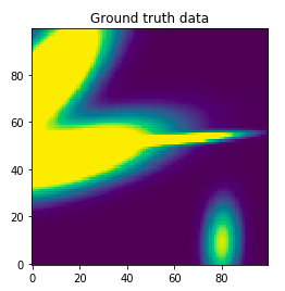
We got ourselves 2 nicely spread gaussians at the left side, another really narrow
one at the middle and another more faint one at the bottom right. This notebook
cell also generated 10,000 train datapoints (randomly sampled from the X input space)
with their true y values and 256 test datapoints.

Let’s see if we can recover the parameters based on X_train and y_train:

First we have to set K (the number of learned gaussians). Recall that our model
assumes we know (or guess) K correctly. I chose K=6 although we generated the
ground truth data with only 4 gaussians, so we can see what happens when there
are “extra” gaussians in the fitted model.

I’m building a simple Keras model, which will have a D size vector as
an input (2D in our case) and a single SumOfGaussians layer. The layer’s output
(the sum of gaussians) will be the model’s output in our case and will be compared
to the y_train data we’ve generated.

Here is the code of the build_model() method:

def build_model(num_learned_gaussians, amps_l1_reg=1e-3, use_means_spread_regularizer=True):
  inp = tf.keras.Input(shape=(NUM_DIMENSIONS,), dtype=tf.float32)

  sog = sog_layer.SumOfGaussians(
      name='sog',
      num_gaussians=num_learned_gaussians,
      amps_l1_reg=amps_l1_reg,
      use_means_spread_regularizer=use_means_spread_regularizer,
      centers_min=[MIN_DATA_VALUE]*NUM_DIMENSIONS, centers_max=[MAX_DATA_VALUE]*NUM_DIMENSIONS,
  )
  out = sog(inp)
  out = Rename('output')(out)  # Rename was defined earlier in the notebook.

  model = tf.keras.Model(
      inputs=inp,
      outputs=out)

  optimizer = tf.keras.optimizers.Adam(learning_rate=1e-3)
  model.compile(optimizer,
               loss={'output': 'mse'},
               metrics={'output': 'mse'})  # this allows returning only the mse without other losses
  return model

Other than the regular Keras model building code, one thing that is worth paying attention
to is the fact that when compiling the model I’m using a multi-head syntax with
only a single head (called output).
This is done because when Keras reports the loss of a model it considers the final
loss together with losses that were created by inner layers in the model (for example

• the L1 loss on the amplitudes and the “centers-spread” loss we use in the
  SumOfGaussians layer).
  When reporting results I only care about the MSE loss, so I gave a name to the
  “regular” output and set a MSE metric on it. That way, when Keras automatically
  reports the total loss and val_loss, it will also report the mse and val_mse
  which will contain only the MSE component of the total loss.

Fitting a model without regularizers

As a first step, let’s fit the model without any additional regularizers (the L1
regularizer that should push unused amplitudes to 0.0 and the pairwise distance
loss that should push centers away from each other). Results can vary a lot with
random initialization, so everything going forward is the output of a single run.
If you run the same Colab yourself, you might get different results.

I’m running for 1000 epochs with the Adam optimizer:

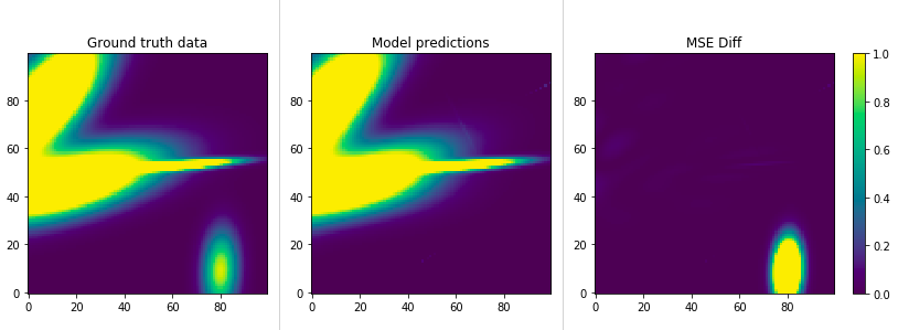
This shows us the ground truth (same as before) on the left, the model’s predictions
in the middle and the diff on the right. We can see that although we completely missed the
gaussian at the bottom right, we’re doing relatively nice work with the others.

The second set of charts shows us the ground truth gaussians vs. the learned ones.
On the side we’ll have the amplitude for each gaussian (both ground truth and learned).
Recall that gaussians with an amplitude close to zero, don’t really affect the
final sum.

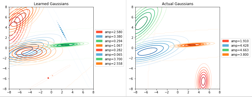
It’s interesting to see how we composed each of the 2 large gaussians on the left
with 2 learned gaussians, that together gave us a similar result. The green learned
gaussian matched almost exactly the orange one and the one on the bottom right was
completely missed. The third chart will give us some hints on why this happened:

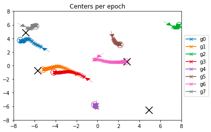
This chart is a bit more complex - we see a “line of x markers” for every gaussian
center, representing its location along the epochs so we can track gaussians
during the training process.
The small arrow shows the initial location (randomly assigned), while the circle
is the final position. The 4 large Xs are the ground truth centers.

We can observe some nice patterns here: The pink one, right in the middle, was
randomly initialized pretty close to one of the real centers, and indeed moves towards
it and ended up exactly on that location. From the last chart (and the actual data
that is shown in the notebook) we can see that it has recovered accurate values
for the center, cov matrix and amplitude for this gaussian.

The red and orange, and the blue and gray ones were both “attracted” to the gaussians
on the left, making the sum of each pair close to the ground truth value (we saw
that earlier in the “Model predictions” heatmap).

Then we have brown, green and purple which were initialized far from real gaussians
and just “got lost” during the process. We can see them in the “Learned Gaussians”
chart (notice that the colors don’t match) but they don’t match any real gaussian and
also have a small amplitude and a vary narrow covariance matrix.

Sadly, no center was initialized next to the gaussian at the bottom right, and no
one was close enough to get a gradient towards it, so it was left alone and can be
considered as a miss of this model.

Fitting a model with regularizers

This time, let’s add both regularizers and see if that changes anything. The
first one is a plain L1 regularizer on the amplitudes vectors. That should help
us eliminate gaussians that are not close to anything as the loss from carrying
their amplitude would be more than the value they produce by reducing the total
MSE. The second one would penalize gaussian centers that are close to each other,
hopefully driving us to a solution where there is a single center for every ground
truth gaussian, and it corresponds to it’s full amplitude value.

Obvisouly, we can play a lot with the regularizers factors. I’m just showing an
example with the default settings, which I must admit, weren’t carefully thought
of…

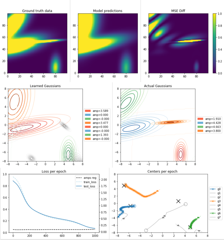
Well, we can see some nice things here, but first, some notations: In the “Learned
Gaussians” and the “Centers per Epoch”, gray lines mean gaussians that ended up
with very small amplitudes (meaning - can be completely ignored).

First, we see how the L1 regularizer helped us eliminate the amplitudes of 5
out of the 8 learned gaussians! Leaving us with a single gaussian learned for 3
of the main ground-truth ones, but completely missing the narrow one in the middle.
This is a problem that’s hard to avoid if the real data contains gaussians
with a very narrow covariance matrix. These gaussians affect a very small area
and probably very few datapoints have fallen in that affected area.
The gradient will throw us in other directions and we’ll completely miss those.
I guess that this is what happened with the small orange gaussian (the
orange one in the ground-truth chart, not the orange center line, sorry for the
colors confusion.. It’s very annoying to make separate charts aligned on the colors…).

We can also see the affect of the centers-pairwise-distances regularizer. Notice
how two centers were initialized very closed to each other and immediately turned
away. Also notice how while the green gaussian got exactly to its closest center
location, the two others that were next to it, turned to different directions as
there was no point in “sharing the amplitude”.

Overall, if we look on the “Learned Gaussians” and “Actual Gaussians” we can see
a nice match on 3 of the gaussians. The forth one is completely missed.

Future work

We saw a problem with narrow gaussians that are easy to miss. In this kind of
setup, here are some ideas to mitigate this:

1. We could run KMeans on the data first, just to get the clusters centers,
   and initialize our gaussians with those centers. We’re more likely then not to
   miss, at least the large centers of datapoints. Notice however, that if our K is
   too small, and there are outlier datapoints, we’ll probably miss those as we’ll
   initialize all centers around the large clusters.

2. Another nice idea is to train with a very high K, and maybe a stronger L1
   regularizer factor. This should allow us to have some centers close to every real
   center, but also “killing” all excess ones through the process. A more advanced
   approach, but a bit more complex to implement, is to start with a very high K,
   and after every N steps, force the least contributing gaussians to a zero
   amplitude while letting the others compensate for the “missing” ones until
   converging at the desired K.

That’s it basically, as always, I’m happy for your comments, fixes, ideas, etc…